The Solvability of the Traveling Salesman Problem

The Solvability of the Traveling Salesman Problem: A Comprehensive Analysis
Executive Summary
The Traveling Salesman Problem (TSP) stands as a foundational challenge in computational science, classified as NP-hard. This classification indicates that no known algorithm can guarantee an optimal solution for all problem instances in polynomial time, signifying a theoretical barrier to universal, efficient exact solutions. Despite this inherent computational complexity, significant practical advancements have been achieved, leading to a nuanced understanding of TSP’s “solvability.”
While a universally efficient exact algorithm remains elusive, the TSP is considered “solved” in a practical sense for a wide range of real-world scenarios. This is accomplished through a strategic combination of highly optimized exact algorithms, which are effective for smaller instances, and advanced heuristic and approximation algorithms, which provide efficient, near-optimal solutions for large-scale problems. Notably, record-breaking instances involving tens of thousands of cities have been solved to optimality using specialized exact methods, demonstrating the power of sophisticated algorithmic engineering. Concurrently, heuristics are indispensable for industries such as logistics, where rapid, actionable solutions are paramount.
The field of TSP research continues its dynamic evolution. Classical optimization techniques are undergoing continuous refinement, while emerging approaches, including deep learning and reinforcement learning, offer novel avenues for developing improved heuristics. This ongoing research underscores that “solving” the TSP is not a static achievement but a continuous process of developing more efficient, robust, and adaptable algorithms to address the complex and evolving demands of real-world optimization challenges.
1. Introduction to the Traveling Salesman Problem (TSP)
1.1 Definition and Fundamental Objective
The Traveling Salesman Problem (TSP) is a classic minimum cost network flow problem rooted in mathematical programming and graph theory. At its core, the problem involves a hypothetical salesman, a defined set of destinations (often referred to as cities), and the known distances or costs associated with traveling between each pair of these destinations. The fundamental objective of the TSP is to determine the shortest possible path that visits each specified destination exactly once and ultimately returns to the initial starting point.
While the original formulation of the TSP primarily focuses on minimizing the total distance traveled, the concept of “cost” can be expanded to encompass various other criteria. For instance, alternative objectives might include minimizing travel time, fuel consumption, or even maximizing revenue in a variant known as the maximum revenue network flow problem, thereby enhancing managerial decision-making beyond simple distance reduction. The overarching goal remains to identify the most efficient route from a multitude of possibilities, thereby minimizing overall travel expenditure. This problem has been a subject of intensive study for over 150 years, continuing to be a prominent area of research.
1.2 Graph Theoretical Formulation
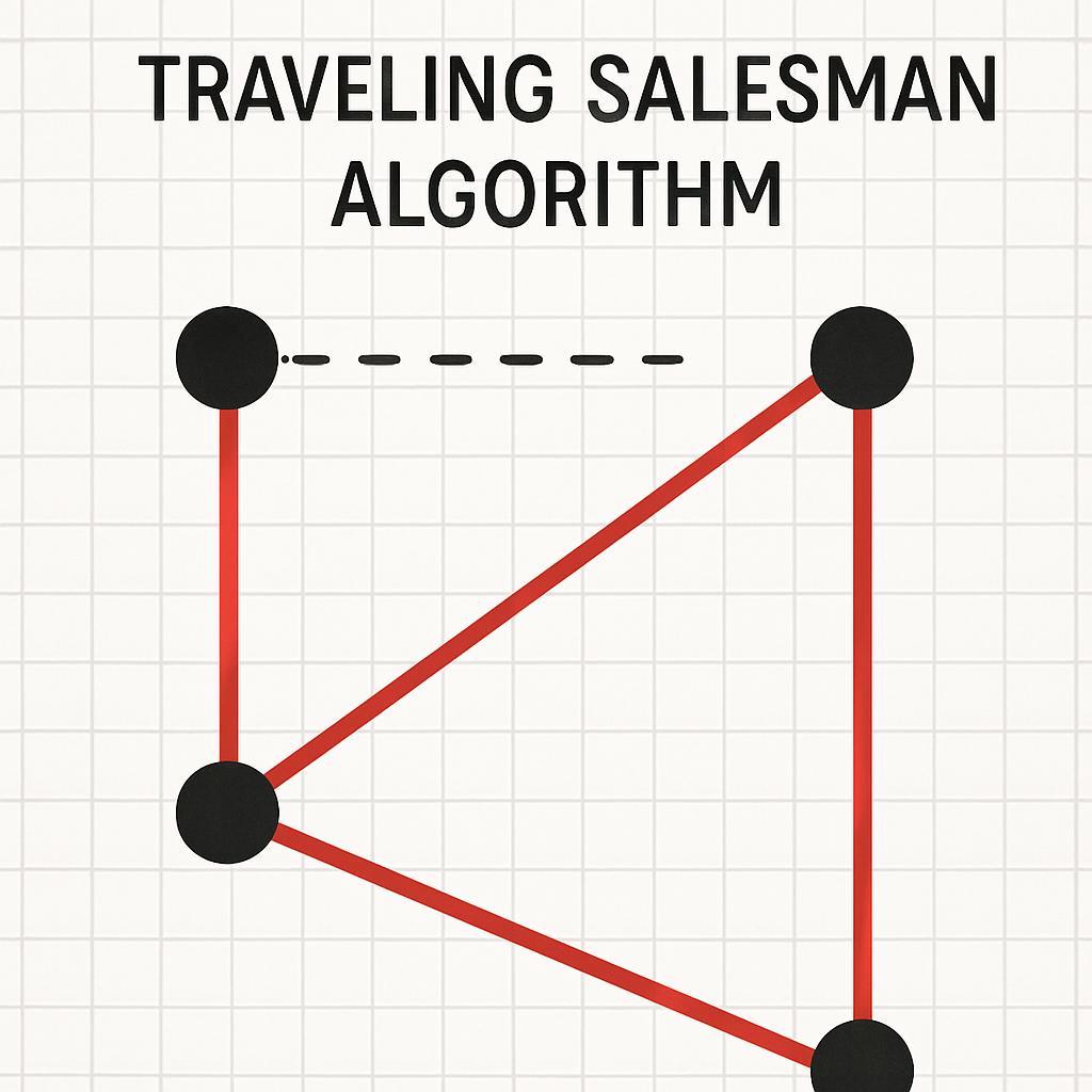
From a mathematical perspective, the TSP is elegantly formulated as a graph problem. In this representation, each city or destination is conceptualized as a node (or vertex), and the distances or costs between these cities are represented as weighted edges connecting the respective nodes. The central challenge then transforms into identifying the optimal Hamiltonian cycle within this weighted graph. A Hamiltonian cycle is defined as a path that commences at a specific vertex, traverses every other vertex exactly once, and concludes by returning to the starting vertex.
The standard TSP model typically assumes a complete graph, denoted as G = (V, E), where V represents the set of ‘n’ vertices (cities), and E signifies the set of edges, each representing the distance between two cities. The problem can manifest in different forms: a symmetric TSP implies that the distance between any two cities is identical regardless of the direction of travel, whereas an asymmetric TSP accounts for potential differences in travel cost or distance depending on the direction.
1.3 Significance and Broad Real-World Relevance
The Traveling Salesman Problem is recognized as one of the most extensively investigated computational problems within the field of optimization. Its status as a benchmark problem allows it to serve as a crucial testbed for evaluating the efficacy of numerous other optimization methodologies. Beyond its academic importance, the TSP possesses profound practical relevance, finding widespread application across diverse sectors. Businesses, governmental bodies, and military organizations actively seek solutions to the TSP to enhance the efficiency of their supply chains and significantly reduce logistical expenditures.
The broad applicability of TSP extends to critical areas such as logistics and supply chain management, where it optimizes delivery routes for companies like FedEx and UPS; urban planning, aiding in the design of efficient public transportation systems; and telecommunications, where it is used to optimize network layouts. Furthermore, its principles are applied in manufacturing for optimizing machine movements, in robotics for planning autonomous vehicle routes, in bioinformatics for DNA sequencing, and even in tour planning for creating efficient itineraries. Emergency services rely on TSP to determine the fastest routes to incidents, and municipalities use it for optimizing waste collection routes, underscoring its pivotal role in minimizing travel distance, saving time, and reducing fuel costs across a myriad of real-world operations.
The pervasive nature of TSP applications in various industries, despite its known theoretical computational hardness, highlights a fundamental aspect of its “solvability” in practice. If the problem were truly intractable, these widespread applications would either not exist or would be demonstrably ineffective. This observation suggests that for many practical purposes, the pursuit of an “optimal” solution in the strictest mathematical sense is often not the sole or primary objective. Instead, the ability to find a “good enough” or “near-optimal” solution efficiently holds substantial practical value and is often sufficient to address real-world needs. This divergence between the theoretical pursuit of absolute optimality and the practical demands of industry, which prioritize actionable, efficient, and cost-effective solutions—even if approximate—lays the groundwork for understanding the critical importance of heuristic and approximation algorithms in addressing the TSP.
2. The Core Challenge: TSP’s NP-Hard Nature
2.1 Explanation of Computational Complexity Classes (P, NP, NP-hard, NP-complete)
To comprehend the inherent difficulty of the Traveling Salesman Problem, it is essential to understand the fundamental classifications within computational complexity theory.
P (Polynomial Time): This class encompasses problems that can be solved by a deterministic computer in polynomial time. This means that as the size of the problem (e.g., the number of cities in TSP) increases, the time required to solve it grows as a polynomial function of the input size (e.g., n, n², n³), indicating efficient solvability.
NP (Non-deterministic Polynomial Time): This class includes problems for which a given solution can be verified in polynomial time by a deterministic computer. In essence, if one is presented with a potential solution, it can be quickly checked for correctness. The term “Non-Deterministic” refers to a theoretical computer that can explore all possible branches of a computation simultaneously.
NP-hard: Informally, NP-hard problems are considered those that are at least as difficult as the hardest problems in NP. More formally, a problem is NP-hard if every problem in NP can be reduced to it in polynomial time. This implies that if an efficient (polynomial-time) algorithm were found for an NP-hard problem, then all problems in NP could also be solved efficiently.
NP-complete: This is a critical subclass within NP-hard problems. NP-complete problems are those that are both NP-hard and also belong to the class NP. Boolean satisfiability (SAT) is a canonical example of an NP-complete problem, and proving that a problem is NP-complete often involves demonstrating a polynomial-time transformation from SAT to that problem.
2.2 Why TSP is Classified as NP-hard
The Traveling Salesman Problem is classified as NP-hard due to the exponential growth of its computational complexity as the number of destinations increases. This inherent complexity means that there is no known polynomial-time algorithm capable of solving it for all instances.
The core difficulty stems from the combinatorial explosion of possible routes. As the number of destinations grows, the corresponding number of unique round-trip routes increases at an exponential rate, quickly exceeding the computational capabilities of even the fastest modern computers. For example, a modest set of ten destinations can result in over 300,000 permutations and combinations of routes, while increasing the number to fifteen destinations yields more than 87 billion possible routes. An exhaustive search, which involves calculating and comparing all possible routes to identify the shortest one, becomes computationally infeasible very rapidly. The NP-hardness of the TSP was formally established by Karp in 1972.
2.3 Distinction Between TSP Optimization and TSP Decision Problems
A crucial technical distinction exists in the formal classification of the Traveling Salesman Problem within computational complexity theory, particularly between its optimization and decision variants.
TSP Optimization (Minimization): This is the most common and intuitive formulation of the problem, where the objective is to find the shortest possible tour that visits all cities exactly once and returns to the origin. This version of the TSP is classified as NP-hard. Importantly, the TSP Optimization problem is not considered to be in the class NP. The reason for this lies in the verification process: if one is provided with a proposed solution (a tour), verifying that it is indeed the shortest possible tour for a given set of cities requires effectively solving the entire TSP, which itself takes exponential time. Consequently, this problem is formally categorized as Opt-P-complete, a complexity class designed to capture optimization problems.
TSP Decision: To fit the formal definition of NP-completeness, problems must typically be “decision problems,” meaning they require a yes/no answer. A simple variation of the TSP transforms it into a decision problem: instead of finding the shortest loop, the goal is to determine if there exists any loop whose total length is less than or equal to some predefined value (e.g., “Is there a tour through all these cities with a total distance less than 100 km?”). This decision variant is classified as NP-complete. If a proposed path is given, it can be verified in polynomial time (specifically, linear time) simply by summing the distances of its edges to check if the total is within the specified bound. The NP-completeness of this decision variant is often demonstrated through a straightforward reduction from the Hamiltonian Cycle problem. While distinct, these two forms of TSP are closely related in terms of complexity: the TSP Minimization problem can be solved by repeatedly calling a TSP Decision oracle through a binary search approach, implying that they are effectively of the same complexity class.
The meticulous differentiation between TSP (optimization) as NP-hard (and Opt-P-complete) and TSP (decision) as NP-complete is a subtle yet critical technicality in computational complexity. The fact that this distinction is sometimes overlooked, even in academic settings, leading to the general statement that “TSP is NP-complete” without further context, highlights a broader challenge in conveying precise computational concepts. The common understanding often simplifies this theoretical nuance, potentially obscuring important implications regarding problem verification and the nature of “solving” an NP-hard problem. A thorough understanding of this distinction is essential for a precise and expert-level discussion of the TSP’s computational landscape.
3. Exact Algorithms: Guaranteeing Optimality (for Small Instances)
Exact algorithms for the Traveling Salesman Problem are designed to find the absolute optimal solution, guaranteeing the shortest possible route. However, their computational demands rapidly escalate with problem size, limiting their practical applicability to instances with a small number of cities.
3.1 Brute-Force Approach
The brute-force approach is the most straightforward exact method for solving the TSP. It operates by systematically generating and evaluating every single possible permutation of routes that visit all destinations, subsequently comparing their total distances to identify the shortest unique solution. This method inherently guarantees the optimal solution because it explores the entire solution space.
Despite its guarantee of optimality, the brute-force approach is severely limited by its computational complexity. Its time complexity is factorial, expressed as O(n!), where ‘n’ represents the number of cities. This factorial growth renders it impractical for even moderately sized instances; for example, it becomes infeasible for problems with more than 20 cities. While a problem with 5 cities might yield a manageable 120 possible permutations, allowing for feasible computation, the rapid increase in permutations quickly surpasses computational capabilities as ‘n’ grows.
3.2 Dynamic Programming (e.g., Held-Karp Algorithm)
Dynamic programming offers a more efficient exact approach compared to brute-force for solving the TSP. This method, exemplified by the Held-Karp algorithm, works by breaking the larger problem into smaller, overlapping subproblems. It solves these subproblems once and stores their results, thereby avoiding redundant calculations when the same subproblems are encountered again. This systematic approach leads to a more efficient computation while still providing an exact, optimal solution.
However, despite its improvements over brute-force, dynamic programming for TSP still exhibits exponential time complexity, typically O(n² * 2^n). This exponential growth means that while it performs significantly better than brute-force, it remains impractical for a large number of cities. Consequently, dynamic programming is generally practical only for small to medium-sized instances, typically those with fewer than 20 cities.
3.3 Branch and Bound
The Branch and Bound algorithm is another powerful exact method employed for TSP. It systematically explores the search space for the optimal solution by intelligently dividing the problem into a series of smaller subproblems. A key feature of this method is its use of “bounding functions” or “pruning techniques.” These techniques allow the algorithm to estimate a lower bound on the cost of any solution that could be found within a particular subproblem. If this lower bound exceeds the cost of the best solution found so far, that entire branch of the search tree can be “pruned” or eliminated, as it cannot possibly lead to an optimal solution. This pruning significantly reduces the overall search space, making Branch and Bound capable of solving larger instances than brute-force. Nevertheless, for very large TSP instances, it can still be computationally intensive and slow.
3.4 Limitations and Practical Thresholds for Exact Solutions
While exact algorithms provide the undeniable advantage of guaranteeing the optimal solution, their inherent computational complexity imposes severe limitations on their applicability. As the number of cities increases, the time required to compute an exact solution grows exponentially, rendering these methods impractical for large-scale instances. The practical thresholds are quite low: brute-force is limited to problems with fewer than 10 cities, and dynamic programming to fewer than 20 cities. Beyond these relatively small numbers, the computational resources and time required become prohibitive.
This consistent observation across various exact algorithms highlights a critical point: while theoretical optimality is desirable, its practical value rapidly diminishes with increasing problem size. The computational burden associated with finding an exact solution for large instances forces a fundamental shift in strategy. This establishes a clear boundary for the applicability of exact methods, underscoring that the “solution” to TSP for most real-world, large-scale problems cannot solely rely on these approaches. Instead, it necessitates the development and adoption of approximate methods, emphasizing that “solving” TSP is not a singular concept but depends heavily on the acceptable trade-off between absolute optimality and computational feasibility within a given timeframe. The choice of algorithm, therefore, becomes highly dependent on the specific requirements of the problem at hand; if an exact solution is absolutely crucial, these algorithms are employed despite their computational limitations.
4. Heuristic and Approximation Algorithms: Practical Solutions for Large Instances
Given the computational intractability of exact algorithms for large-scale TSP instances, heuristic and approximation algorithms emerge as indispensable tools. These methods do not guarantee the absolute optimal solution but are designed to provide high-quality, “good enough” solutions within a reasonable and practical timeframe. They achieve this by employing intelligent strategies and approximate techniques to efficiently explore the vast solution space.
Table 1: Comparison of TSP Algorithm Types
Algorithm Type
Solution Quality
Computational Efficiency
Suitability/Best For
Exact
Optimal
Impractical for large
Small instances
Heuristic
Near-optimal/Satisfactory
Reasonable time
Large instances
Approximation
Guaranteed Approximation
Efficient
Specific problem types (e.g., metric TSP)

4.1 Heuristics
Heuristic algorithms are problem-solving techniques that employ practical methods not guaranteed to be optimal or perfect, but sufficient for reaching an immediate, short-term goal. For TSP, they provide satisfactory results quickly.
Nearest Neighbor Algorithm: This is arguably the simplest heuristic approach to the TSP. The method involves starting at a random city, then repeatedly moving to the nearest unvisited city until all destinations have been visited, finally returning to the initial starting point. Its time complexity is relatively low, typically O(n²). The primary advantages of the Nearest Neighbor algorithm are its simplicity and speed. However, its main disadvantage is that the solution it generates may not be very close to the optimal route, and it lacks a constant approximation ratio for the general metric TSP.
Greedy Algorithm: The greedy algorithm for TSP operates by, at each step, selecting the shortest available edge between cities without forming a premature cycle that excludes other cities. This method is quick and simple, with a time complexity of O(n² log n). Similar to Nearest Neighbor, its main drawback is that it does not guarantee the shortest possible route.
Lin-Kernighan Heuristic (LKH): The Lin-Kernighan heuristic is a sophisticated local search algorithm designed to improve the quality of a tour by iteratively exchanging edges. It is widely regarded as one of the most effective and well-known algorithms for solving symmetric and asymmetric TSP instances, particularly for large-scale problems. LKH can be applied effectively to problems with over 100,0